A spectrum analyzer is a phenomenally useful piece of test equipment when working on RF circuitry. While used, several generation old spectrum analyzers can be found fairly reasonably priced, network analyzers are usually out of reach for a home lab. However, with a little bit of additional equipment some of the measurements that would normally require a network analyzer can be done on a spectrum analyzer.
The example I will be using is measuring the insertion loss and bandwidth of a 10 GHz cavity filter.
Since a spectrum analyzer is a passive device, a source of RF energy is the main thing needed to perform these measurements. Sometimes a tracking generator can be had as an option for your spectrum analyzer. A tracking generator is basically an oscillator that tracks along with the frequency as the spectrum analyzer sweeps its set range. However, the one available for my spectrum analyzer only goes up to a few GHz.
Another more brute force approach is an RF noise source. These are available in a few different forms, both solid state, like the HP 346B, and with a pulsed gas discharge tube. The solid state ones are usually pretty expensive, while the gas discharge ones are large and have specific power requirements. Also, depending on your system noise level, the noise sources may be too weak to make meaningful measurements with.
Why not use something you probably already have: an oscillator? Repeatedly sweeping the oscillator across a band of interest, in combination with the peak hold feature on the spectrum analyzer, produces a result similar to a noise source!
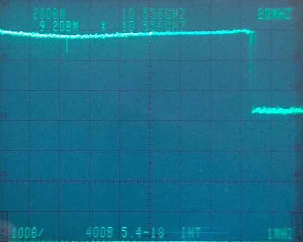
Here I used my mystery YIG oscillator and a function generator with a power transistor to sweep approximately 200 MHz around 10.5 GHz. With the peak hold turned off, a few spikes can be seen dancing around the screen. After turning it on, the curve below starts to fill in. Depending on the sweep speed, span, etc. this can take 20-30 seconds. However, the shapes of the curves being traced out are readily apparently long before the curves are completely filled in. For this simple experiment, I just made a note of the power level and flatness. For more accurate measurements later, this trace could be downloaded from the instrument.
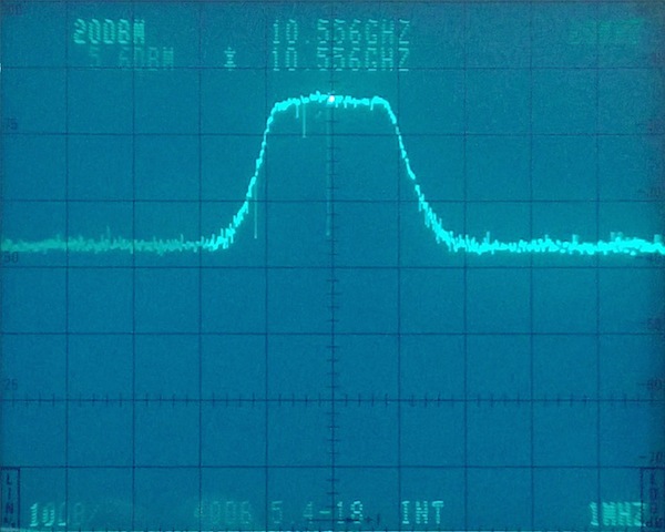
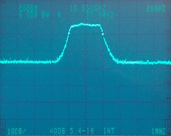
After I had a baseline trace, I put the filter in the circuit and turned on the oscillator. Thirty seconds later I had the passband of the filter! I could then make measurements like the insertion loss (3.6 dB, which seems high but is probably related to cabling), and bandwidth (around 35 MHz, as expected). In the first photo, there are still a few points that haven't filled in, but by the second photo they have. If the baseline trace was saved, this trace could now be subtracted from it to give loss vs. frequency.

Baseline swept signal saved for future comparison. 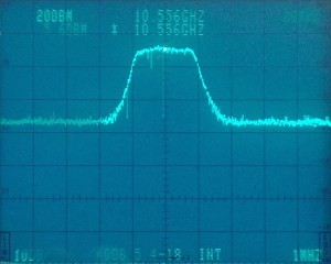
Passband trace on 4-section cavity filter tuned for 10556 MHz. 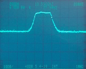
Bandwidth measurement on 4-section cavity filter tuned for 10556 MHz.